Is Guess = Read Default for Geom = Checkpoint
Data visualisation
Introduction
"The uncomplicated graph has brought more information to the data analyst's heed than whatsoever other device." — John Tukey
This chapter will teach y'all how to visualise your data using ggplot2. R has several systems for making graphs, but ggplot2 is one of the nigh elegant and most versatile. ggplot2 implements the grammar of graphics, a coherent organisation for describing and building graphs. With ggplot2, you can do more faster past learning 1 system and applying it in many places.
If you'd similar to learn more nigh the theoretical underpinnings of ggplot2 before y'all start, I'd recommend reading "The Layered Grammer of Graphics", http://vita.had.co.nz/papers/layered-grammar.pdf.
Prerequisites
This chapter focusses on ggplot2, one of the cadre members of the tidyverse. To access the datasets, assist pages, and functions that we will utilize in this chapter, load the tidyverse by running this code:
library ( tidyverse ) #> ── Attaching packages ─────────────────────────────────────── tidyverse 1.3.0 ── #> ✔ ggplot2 3.3.2 ✔ purrr 0.3.4 #> ✔ tibble 3.0.iii ✔ dplyr 1.0.2 #> ✔ tidyr 1.1.2 ✔ stringr 1.four.0 #> ✔ readr 1.4.0 ✔ forcats 0.v.0 #> ── Conflicts ────────────────────────────────────────── tidyverse_conflicts() ── #> ✖ dplyr::filter() masks stats::filter() #> ✖ dplyr::lag() masks stats::lag() That one line of code loads the core tidyverse; packages which you will use in almost every data assay. It also tells you which functions from the tidyverse conflict with functions in base R (or from other packages yous might have loaded).
If you run this code and become the error bulletin "there is no package called 'tidyverse'", y'all'll need to first install it, then run library() in one case again.
You just need to install a packet once, but you need to reload it every fourth dimension you start a new session.
If nosotros need to be explicit virtually where a role (or dataset) comes from, nosotros'll utilize the special course packet::role(). For example, ggplot2::ggplot() tells you explicitly that we're using the ggplot() function from the ggplot2 bundle.
Get-go steps
Let's use our starting time graph to answer a question: Do cars with big engines use more fuel than cars with minor engines? Y'all probably already have an reply, but endeavour to brand your answer precise. What does the relationship betwixt engine size and fuel efficiency look like? Is it positive? Negative? Linear? Nonlinear?
The mpg data frame
You lot can test your reply with the mpg data frame found in ggplot2 (aka ggplot2::mpg). A information frame is a rectangular collection of variables (in the columns) and observations (in the rows). mpg contains observations collected by the Us Environmental Protection Agency on 38 models of car.
mpg #> # A tibble: 234 x eleven #> manufacturer model displ year cyl trans drv cty hwy fl class #> <chr> <chr> <dbl> <int> <int> <chr> <chr> <int> <int> <chr> <chr> #> 1 audi a4 1.8 1999 4 car(l5) f eighteen 29 p compa… #> 2 audi a4 1.8 1999 iv manual(m5) f 21 29 p compa… #> three audi a4 2 2008 iv manual(m6) f 20 31 p compa… #> 4 audi a4 2 2008 iv car(av) f 21 30 p compa… #> five audi a4 ii.eight 1999 6 auto(l5) f 16 26 p compa… #> six audi a4 2.eight 1999 6 manual(m5) f 18 26 p compa… #> # … with 228 more than rows Amid the variables in mpg are:
-
displ, a car'due south engine size, in litres. -
hwy, a car's fuel efficiency on the highway, in miles per gallon (mpg). A car with a depression fuel efficiency consumes more fuel than a car with a high fuel efficiency when they travel the same distance.
To learn more nearly mpg, open its help page past running ?mpg.
Creating a ggplot
To plot mpg, run this code to put displ on the x-axis and hwy on the y-axis:
ggplot (information = mpg ) + geom_point (mapping = aes (x = displ, y = hwy ) ) 
The plot shows a negative human relationship between engine size (displ) and fuel efficiency (hwy). In other words, cars with big engines utilize more than fuel. Does this confirm or refute your hypothesis almost fuel efficiency and engine size?
With ggplot2, y'all begin a plot with the function ggplot(). ggplot() creates a coordinate system that you tin can add layers to. The first argument of ggplot() is the dataset to use in the graph. Then ggplot(data = mpg) creates an empty graph, but information technology'due south not very interesting so I'thou not going to show it here.
You complete your graph by adding one or more than layers to ggplot(). The role geom_point() adds a layer of points to your plot, which creates a scatterplot. ggplot2 comes with many geom functions that each add together a dissimilar blazon of layer to a plot. You'll learn a whole bunch of them throughout this chapter.
Each geom role in ggplot2 takes a mapping statement. This defines how variables in your dataset are mapped to visual properties. The mapping argument is always paired with aes(), and the x and y arguments of aes() specify which variables to map to the x and y axes. ggplot2 looks for the mapped variables in the data argument, in this example, mpg.
A graphing template
Permit's turn this code into a reusable template for making graphs with ggplot2. To make a graph, supersede the bracketed sections in the code beneath with a dataset, a geom function, or a drove of mappings.
ggplot(information = <DATA>) + <GEOM_FUNCTION>(mapping = aes(<MAPPINGS>)) The rest of this chapter will bear witness yous how to complete and extend this template to make different types of graphs. We will begin with the <MAPPINGS> component.
Exercises
-
Run
ggplot(information = mpg). What practice you lot see? -
How many rows are in
mpg? How many columns? -
What does the
drvvariable draw? Read the help for?mpgto find out. -
Brand a scatterplot of
hwyvscyl. -
What happens if you make a scatterplot of
classvsdrv? Why is the plot not useful?
Aesthetic mappings
"The greatest value of a motion picture is when it forces united states of america to notice what we never expected to come across." — John Tukey
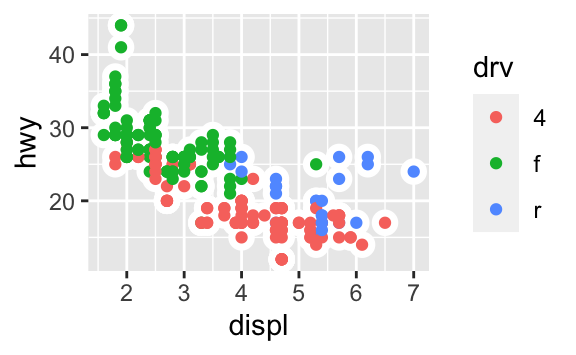
In the plot below, ane group of points (highlighted in red) seems to fall exterior of the linear trend. These cars have a higher mileage than you might expect. How can you explain these cars?
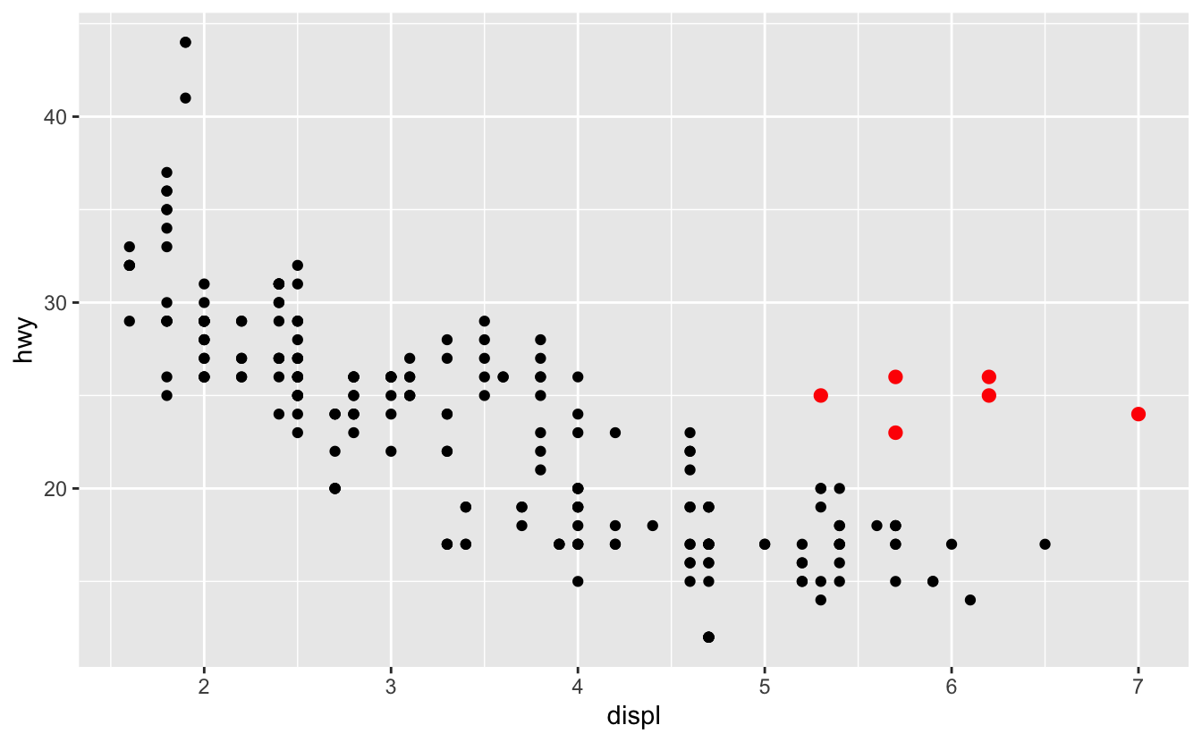
Let's hypothesize that the cars are hybrids. One way to test this hypothesis is to look at the class value for each automobile. The class variable of the mpg dataset classifies cars into groups such equally meaty, midsize, and SUV. If the outlying points are hybrids, they should exist classified as compact cars or, maybe, subcompact cars (proceed in mind that this information was collected before hybrid trucks and SUVs became popular).
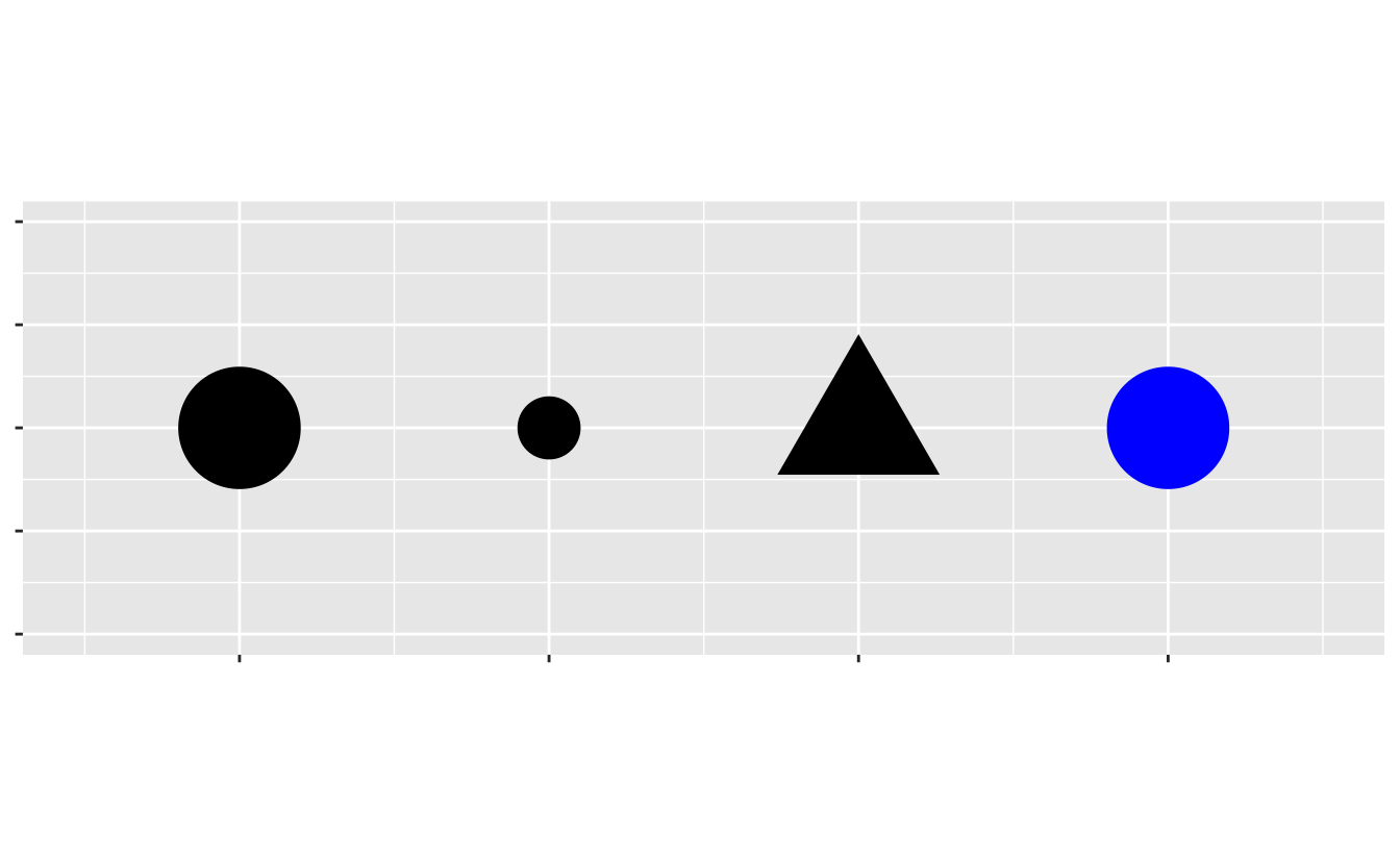
You can add together a third variable, like class, to a two dimensional scatterplot past mapping information technology to an artful. An artful is a visual property of the objects in your plot. Aesthetics include things like the size, the shape, or the color of your points. You can display a signal (like the 1 beneath) in different means by changing the values of its artful properties. Since we already utilize the word "value" to describe data, let'south use the word "level" to describe aesthetic properties. Here we change the levels of a betoken'south size, shape, and color to make the bespeak minor, triangular, or bluish:
You can convey information about your information by mapping the aesthetics in your plot to the variables in your dataset. For example, you can map the colors of your points to the course variable to reveal the class of each car.
ggplot (data = mpg ) + geom_point (mapping = aes (x = displ, y = hwy, color = class ) ) 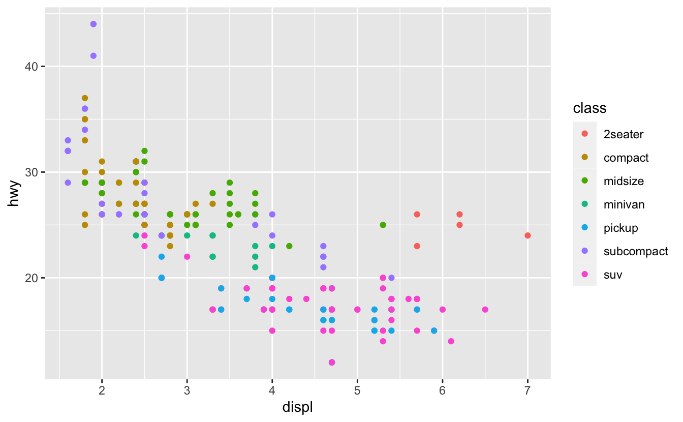
(If yous prefer British English, like Hadley, y'all tin can use colour instead of color.)
To map an aesthetic to a variable, associate the proper name of the aesthetic to the name of the variable inside aes(). ggplot2 will automatically assign a unique level of the artful (here a unique color) to each unique value of the variable, a process known equally scaling. ggplot2 will also add a legend that explains which levels correspond to which values.
The colors reveal that many of the unusual points are two-seater cars. These cars don't seem like hybrids, and are, in fact, sports cars! Sports cars accept large engines similar SUVs and pickup trucks, but small bodies like midsize and compact cars, which improves their gas mileage. In retrospect, these cars were unlikely to be hybrids since they accept big engines.
In the higher up example, we mapped class to the color aesthetic, but nosotros could accept mapped form to the size artful in the same manner. In this case, the exact size of each point would reveal its form affiliation. We get a warning here, because mapping an unordered variable (class) to an ordered aesthetic (size) is not a good idea.
ggplot (data = mpg ) + geom_point (mapping = aes (x = displ, y = hwy, size = class ) ) #> Warning: Using size for a detached variable is not advised. 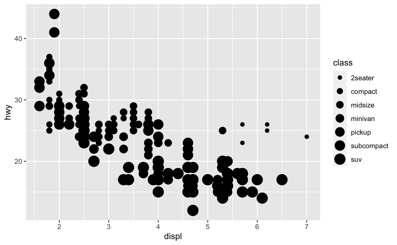
Or we could have mapped class to the alpha artful, which controls the transparency of the points, or to the shape aesthetic, which controls the shape of the points.
# Left ggplot (data = mpg ) + geom_point (mapping = aes (10 = displ, y = hwy, blastoff = course ) ) # Right ggplot (information = mpg ) + geom_point (mapping = aes (ten = displ, y = hwy, shape = class ) ) 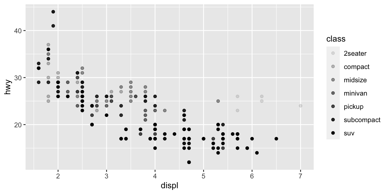
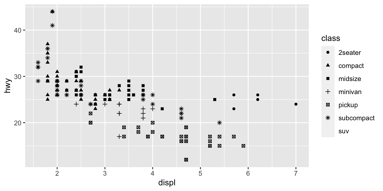
What happened to the SUVs? ggplot2 will only utilise six shapes at a time. By default, additional groups will go unplotted when yous employ the shape artful.
For each artful, you use aes() to associate the name of the aesthetic with a variable to display. The aes() function gathers together each of the artful mappings used by a layer and passes them to the layer's mapping argument. The syntax highlights a useful insight about x and y: the x and y locations of a point are themselves aesthetics, visual properties that yous can map to variables to display information nigh the data.
Once you lot map an aesthetic, ggplot2 takes care of the rest. It selects a reasonable scale to utilize with the aesthetic, and it constructs a legend that explains the mapping between levels and values. For x and y aesthetics, ggplot2 does not create a fable, but it creates an centrality line with tick marks and a characterization. The centrality line acts as a fable; it explains the mapping between locations and values.
Yous can also set the artful properties of your geom manually. For instance, we can make all of the points in our plot blue:
ggplot (data = mpg ) + geom_point (mapping = aes (10 = displ, y = hwy ), color = "blue" ) 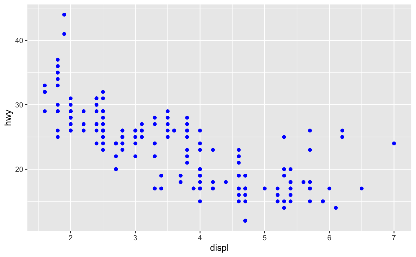
Here, the color doesn't convey information about a variable, but but changes the appearance of the plot. To set up an aesthetic manually, set the aesthetic by proper noun as an statement of your geom function; i.due east. information technology goes outside of aes(). You'll need to option a level that makes sense for that aesthetic:
-
The name of a color equally a character string.
-
The size of a point in mm.
-
The shape of a point every bit a number, equally shown in Effigy 3.ane.
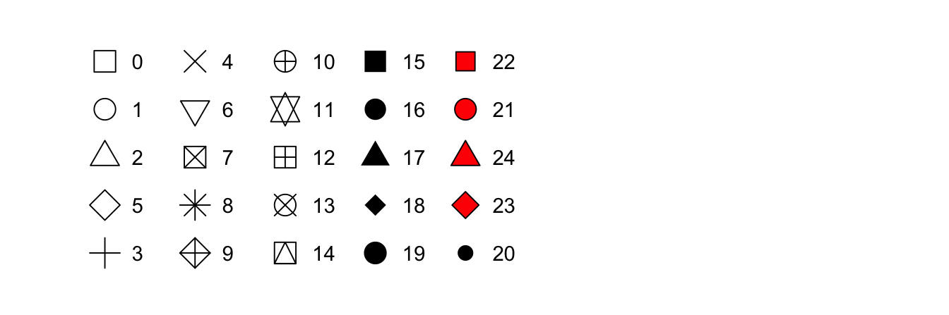
Effigy 3.ane: R has 25 congenital in shapes that are identified past numbers. There are some seeming duplicates: for example, 0, 15, and 22 are all squares. The difference comes from the interaction of the color and fill aesthetics. The hollow shapes (0–14) have a border determined past colour; the solid shapes (xv–20) are filled with colour; the filled shapes (21–24) have a border of color and are filled with fill.
Exercises
-
What's gone wrong with this code? Why are the points not bluish?
ggplot (data = mpg ) + geom_point (mapping = aes (x = displ, y = hwy, color = "bluish" ) )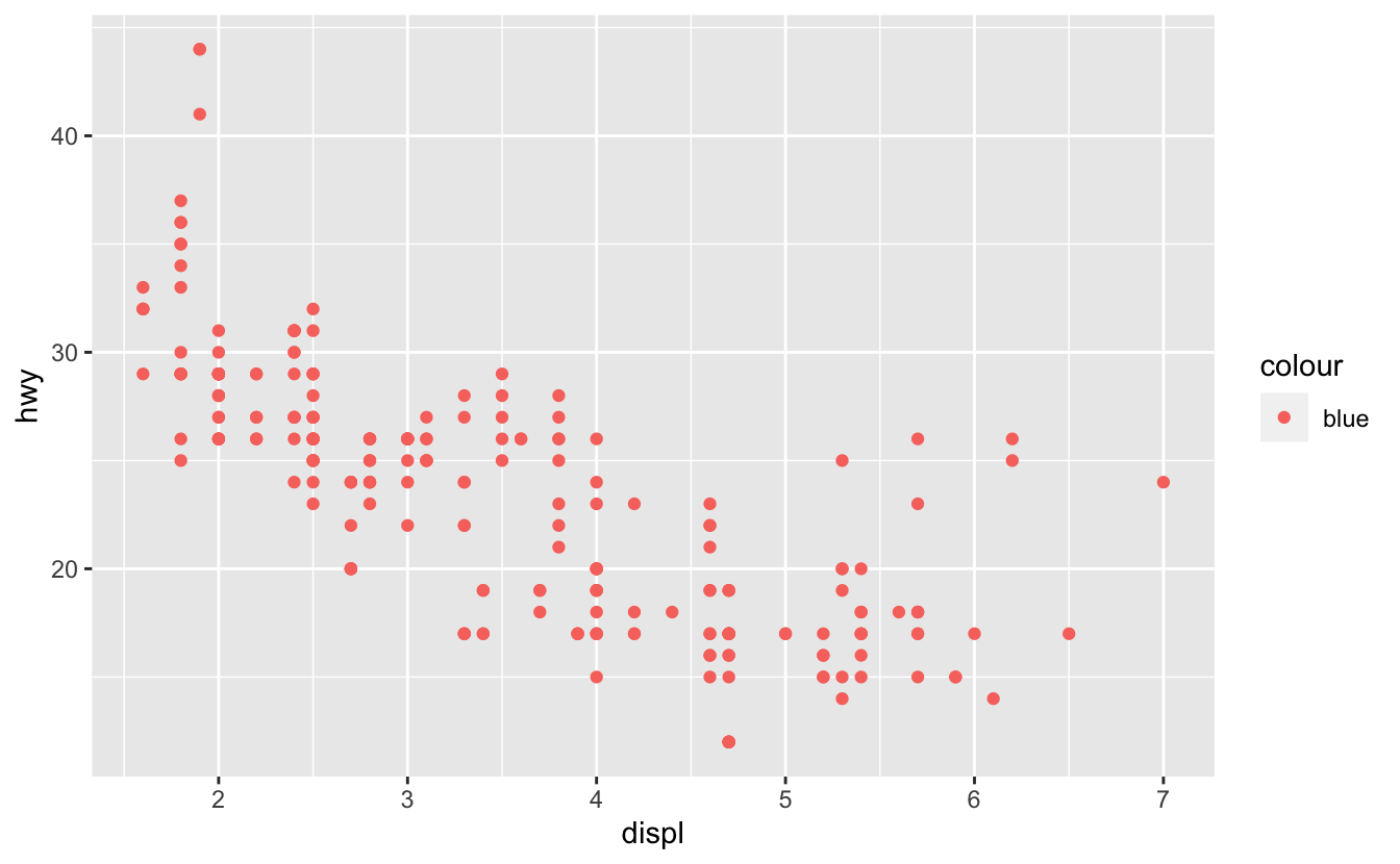
-
Which variables in
mpgare categorical? Which variables are continuous? (Hint: type?mpgto read the documentation for the dataset). How tin can you see this information when you runmpg? -
Map a continuous variable to
color,size, andshape. How exercise these aesthetics deport differently for categorical vs. continuous variables? -
What happens if you map the same variable to multiple aesthetics?
-
What does the
strokeaesthetic do? What shapes does it work with? (Hint: utilize?geom_point) -
What happens if you map an aesthetic to something other than a variable name, similar
aes(colour = displ < 5)? Note, yous'll also demand to specify 10 and y.
Common problems
As you showtime to run R code, you're likely to run into bug. Don't worry — it happens to everyone. I have been writing R code for years, and every twenty-four hour period I still write code that doesn't work!
Start past carefully comparing the lawmaking that you're running to the code in the book. R is extremely picky, and a misplaced character tin make all the difference. Make certain that every ( is matched with a ) and every " is paired with another ". Sometimes you lot'll run the lawmaking and cypher happens. Check the left-hand of your console: if it's a +, it ways that R doesn't think you've typed a complete expression and information technology'southward waiting for you lot to finish it. In this case, it's usually like shooting fish in a barrel to start from scratch again by pressing ESCAPE to arrest processing the current command.
Ane common problem when creating ggplot2 graphics is to put the + in the wrong place: it has to come up at the terminate of the line, not the start. In other words, make sure you haven't accidentally written code like this:
ggplot (information = mpg ) + geom_point (mapping = aes (x = displ, y = hwy ) ) If y'all're however stuck, endeavor the help. You tin get help about any R part past running ?function_name in the console, or selecting the function proper name and pressing F1 in RStudio. Don't worry if the assist doesn't seem that helpful - instead skip downwardly to the examples and expect for code that matches what you're trying to do.
If that doesn't help, carefully read the error message. Sometimes the answer will be buried at that place! Only when you lot're new to R, the respond might be in the fault bulletin but you don't notwithstanding know how to understand it. Another great tool is Google: try googling the fault message, as information technology's likely someone else has had the same problem, and has gotten assist online.
Facets
One way to add additional variables is with aesthetics. Another way, peculiarly useful for categorical variables, is to split your plot into facets, subplots that each brandish one subset of the data.
To facet your plot by a unmarried variable, use facet_wrap(). The first statement of facet_wrap() should be a formula, which you create with ~ followed by a variable name (here "formula" is the name of a data construction in R, not a synonym for "equation"). The variable that you lot pass to facet_wrap() should be discrete.
ggplot (data = mpg ) + geom_point (mapping = aes (x = displ, y = hwy ) ) + facet_wrap ( ~ class, nrow = 2 ) 
To facet your plot on the combination of 2 variables, add facet_grid() to your plot call. The first statement of facet_grid() is also a formula. This time the formula should comprise two variable names separated by a ~.
ggplot (data = mpg ) + geom_point (mapping = aes (ten = displ, y = hwy ) ) + facet_grid ( drv ~ cyl ) 
If you lot prefer to not facet in the rows or columns dimension, use a . instead of a variable proper name, e.g.+ facet_grid(. ~ cyl).
Exercises
-
What happens if you facet on a continuous variable?
-
What do the empty cells in plot with
facet_grid(drv ~ cyl)hateful? How do they relate to this plot?ggplot (data = mpg ) + geom_point (mapping = aes (ten = drv, y = cyl ) ) -
What plots does the following lawmaking brand? What does
.do?ggplot (data = mpg ) + geom_point (mapping = aes (10 = displ, y = hwy ) ) + facet_grid ( drv ~ . ) ggplot (data = mpg ) + geom_point (mapping = aes (x = displ, y = hwy ) ) + facet_grid ( . ~ cyl ) -
Take the first faceted plot in this section:
ggplot (data = mpg ) + geom_point (mapping = aes (x = displ, y = hwy ) ) + facet_wrap ( ~ class, nrow = ii )What are the advantages to using faceting instead of the color artful? What are the disadvantages? How might the rest change if you had a larger dataset?
-
Read
?facet_wrap. What doesnrowpractice? What doesncoldo? What other options control the layout of the individual panels? Why doesn'tfacet_grid()havenrowandncolarguments? -
When using
facet_grid()you should usually put the variable with more than unique levels in the columns. Why?
Geometric objects
How are these 2 plots similar?
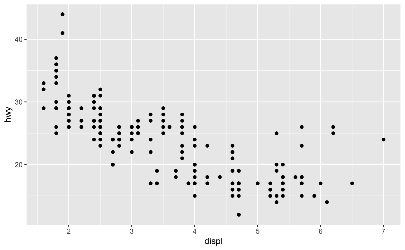
Both plots incorporate the same 10 variable, the same y variable, and both describe the same data. Simply the plots are not identical. Each plot uses a different visual object to represent the data. In ggplot2 syntax, we say that they use different geoms.
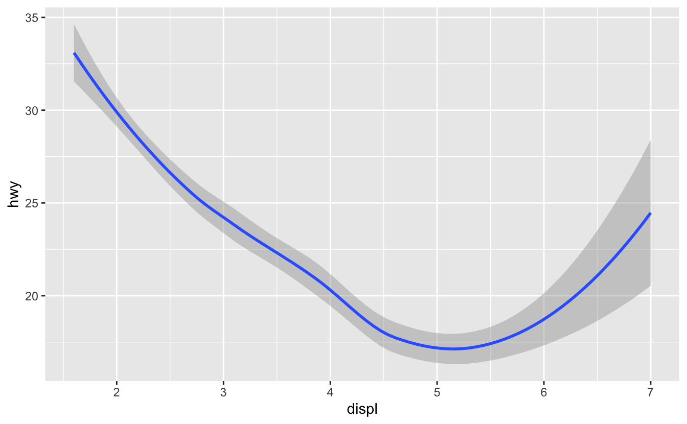
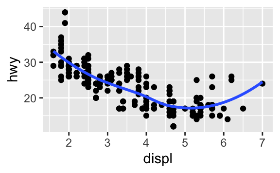
A geom is the geometrical object that a plot uses to represent data. People often draw plots past the type of geom that the plot uses. For example, bar charts use bar geoms, line charts use line geoms, boxplots utilize boxplot geoms, and so on. Scatterplots interruption the trend; they apply the point geom. Equally nosotros see to a higher place, you tin can use unlike geoms to plot the same data. The plot on the left uses the point geom, and the plot on the correct uses the polish geom, a smooth line fitted to the data.
To change the geom in your plot, change the geom role that you add to ggplot(). For example, to brand the plots above, you tin use this lawmaking:
# left ggplot (data = mpg ) + geom_point (mapping = aes (ten = displ, y = hwy ) ) # right ggplot (data = mpg ) + geom_smooth (mapping = aes (x = displ, y = hwy ) ) Every geom function in ggplot2 takes a mapping argument. However, not every aesthetic works with every geom. You could gear up the shape of a bespeak, only y'all couldn't prepare the "shape" of a line. On the other manus, you could set the linetype of a line. geom_smooth() will draw a different line, with a different linetype, for each unique value of the variable that yous map to linetype.
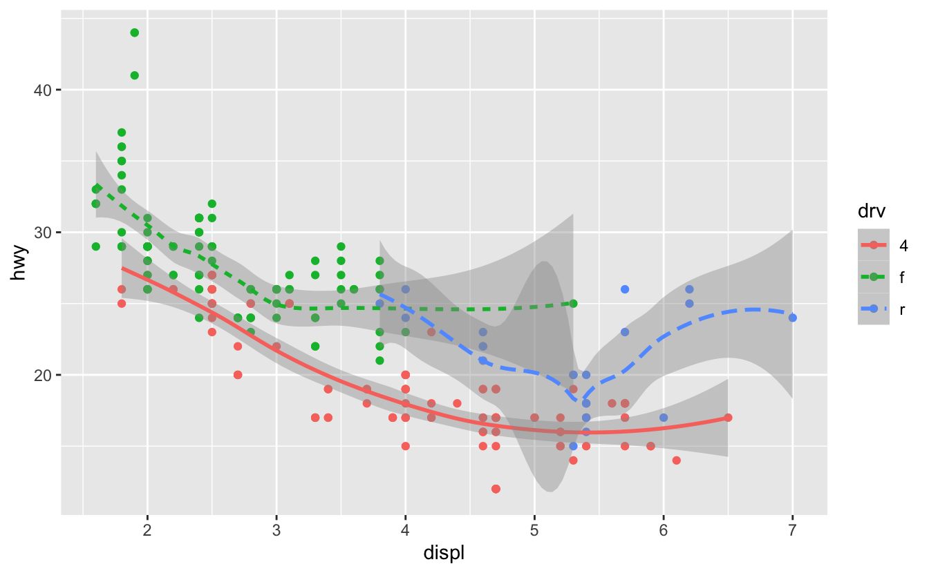
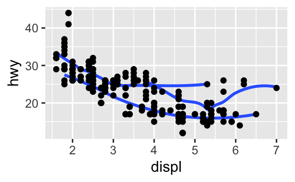
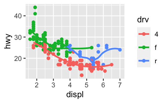
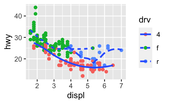
ggplot (data = mpg ) + geom_smooth (mapping = aes (x = displ, y = hwy, linetype = drv ) ) 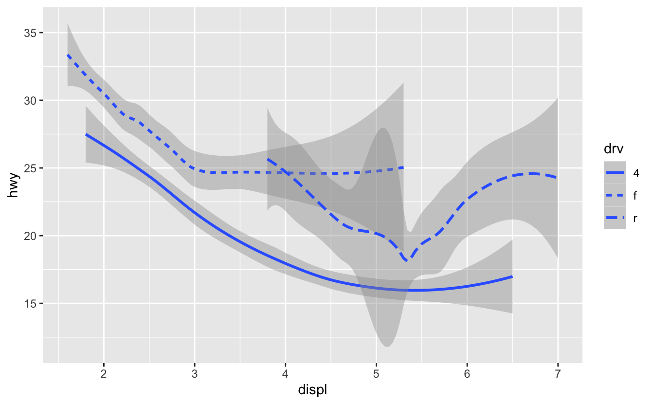
Here geom_smooth() separates the cars into 3 lines based on their drv value, which describes a car's drivetrain. Ane line describes all of the points with a iv value, one line describes all of the points with an f value, and one line describes all of the points with an r value. Here, 4 stands for four-wheel drive, f for front-wheel bulldoze, and r for rear-wheel drive.
If this sounds strange, we can make it more clear by overlaying the lines on top of the raw data and then coloring everything according to drv.
Notice that this plot contains two geoms in the same graph! If this makes you excited, buckle up. We volition learn how to place multiple geoms in the aforementioned plot very soon.
ggplot2 provides over xl geoms, and extension packages provide even more than (meet https://exts.ggplot2.tidyverse.org/gallery/ for a sampling). The best way to get a comprehensive overview is the ggplot2 cheatsheet, which you tin find at http://rstudio.com/resources/cheatsheets. To learn more virtually whatever single geom, use help: ?geom_smooth.
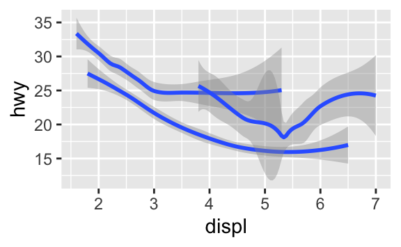
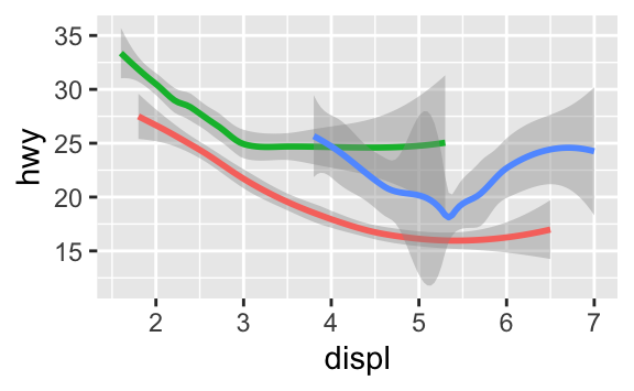
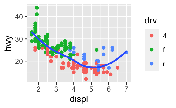
Many geoms, like geom_smooth(), apply a single geometric object to display multiple rows of data. For these geoms, you can set up the group aesthetic to a chiselled variable to draw multiple objects. ggplot2 will draw a separate object for each unique value of the grouping variable. In practice, ggplot2 will automatically group the information for these geoms whenever you map an aesthetic to a discrete variable (every bit in the linetype example). It is user-friendly to rely on this feature because the grouping aesthetic by itself does not add a legend or distinguishing features to the geoms.
ggplot (information = mpg ) + geom_smooth (mapping = aes (x = displ, y = hwy ) ) ggplot (data = mpg ) + geom_smooth (mapping = aes (x = displ, y = hwy, group = drv ) ) ggplot (data = mpg ) + geom_smooth ( mapping = aes (ten = displ, y = hwy, color = drv ), show.legend = FALSE ) 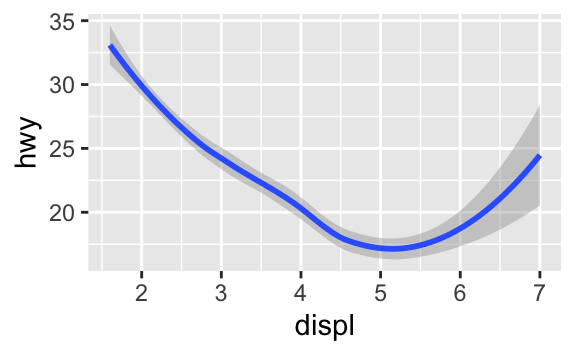
To brandish multiple geoms in the same plot, add multiple geom functions to ggplot():
ggplot (data = mpg ) + geom_point (mapping = aes (x = displ, y = hwy ) ) + geom_smooth (mapping = aes (ten = displ, y = hwy ) ) 
This, nonetheless, introduces some duplication in our code. Imagine if you wanted to alter the y-centrality to display cty instead of hwy. You'd need to change the variable in two places, and you might forget to update one. You tin avert this type of repetition by passing a set of mappings to ggplot(). ggplot2 will care for these mappings as global mappings that utilize to each geom in the graph. In other words, this code will produce the same plot equally the previous lawmaking:
ggplot (data = mpg, mapping = aes (ten = displ, y = hwy ) ) + geom_point ( ) + geom_smooth ( ) If you place mappings in a geom function, ggplot2 will treat them as local mappings for the layer. Information technology volition utilize these mappings to extend or overwrite the global mappings for that layer only. This makes it possible to brandish different aesthetics in different layers.
ggplot (data = mpg, mapping = aes (ten = displ, y = hwy ) ) + geom_point (mapping = aes (colour = class ) ) + geom_smooth ( ) 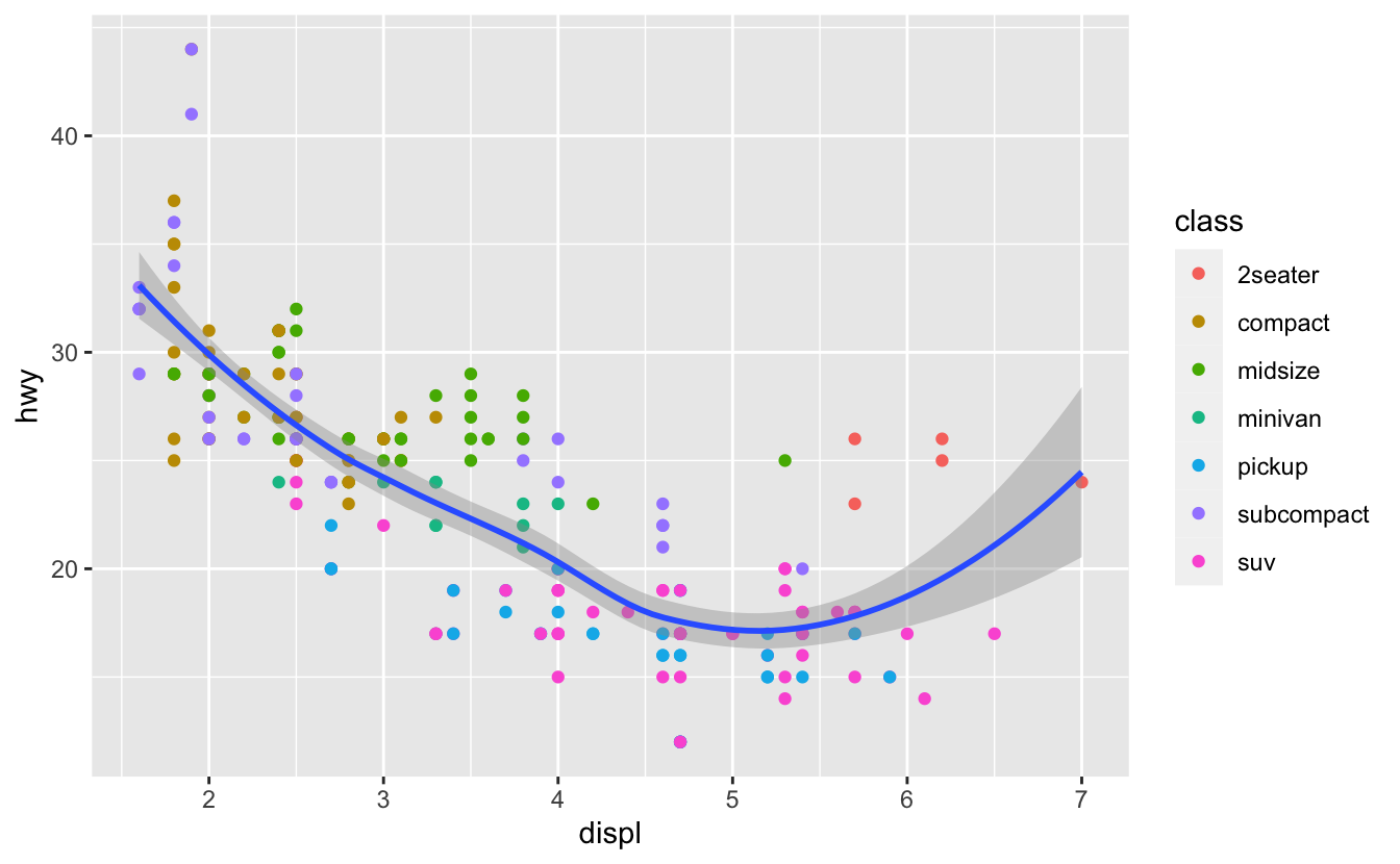
You tin can utilise the same idea to specify unlike data for each layer. Hither, our polish line displays but a subset of the mpg dataset, the subcompact cars. The local data argument in geom_smooth() overrides the global information argument in ggplot() for that layer only.
ggplot (data = mpg, mapping = aes (x = displ, y = hwy ) ) + geom_point (mapping = aes (colour = class ) ) + geom_smooth (data = filter ( mpg, class == "subcompact" ), se = FALSE ) 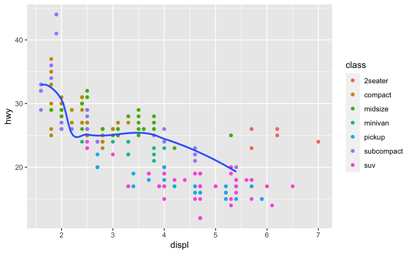
(You'll learn how filter() works in the affiliate on data transformations: for now, but know that this command selects only the subcompact cars.)
Exercises
-
What geom would you utilise to draw a line chart? A boxplot? A histogram? An surface area chart?
-
Run this code in your head and predict what the output will look like. Then, run the code in R and bank check your predictions.
ggplot (information = mpg, mapping = aes (ten = displ, y = hwy, color = drv ) ) + geom_point ( ) + geom_smooth (se = Faux ) -
What does
bear witness.legend = FALSEdo? What happens if you remove it?
Why do you think I used it earlier in the chapter? -
What does the
sestatement togeom_smooth()do? -
Will these two graphs await unlike? Why/why not?
ggplot (data = mpg, mapping = aes (x = displ, y = hwy ) ) + geom_point ( ) + geom_smooth ( ) ggplot ( ) + geom_point (information = mpg, mapping = aes (x = displ, y = hwy ) ) + geom_smooth (data = mpg, mapping = aes (10 = displ, y = hwy ) ) -
Recreate the R code necessary to generate the following graphs.
Statistical transformations
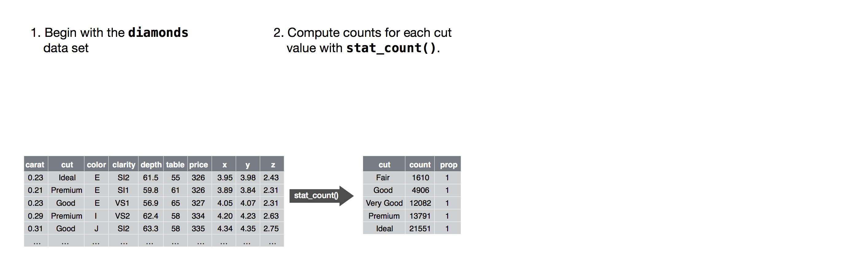
Next, let's take a await at a bar chart. Bar charts seem simple, but they are interesting because they reveal something subtle about plots. Consider a basic bar chart, as drawn with geom_bar(). The following chart displays the total number of diamonds in the diamonds dataset, grouped by cut. The diamonds dataset comes in ggplot2 and contains data about ~54,000 diamonds, including the price, carat, color, clarity, and cutting of each diamond. The chart shows that more than diamonds are available with loftier quality cuts than with low quality cuts.
ggplot (data = diamonds ) + geom_bar (mapping = aes (x = cut ) ) 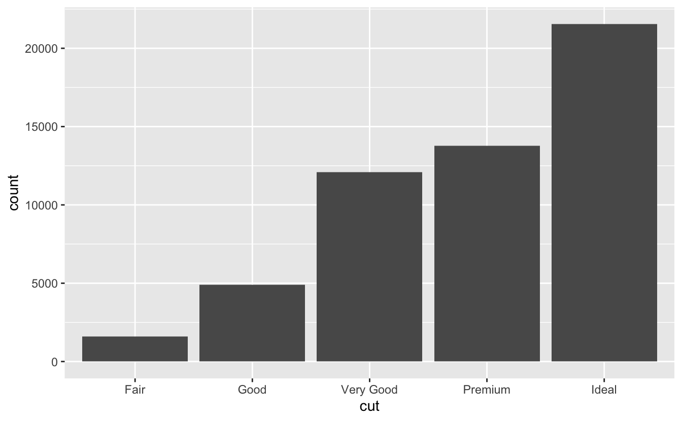
On the 10-centrality, the chart displays cutting, a variable from diamonds. On the y-axis, it displays count, only count is not a variable in diamonds! Where does count come from? Many graphs, like scatterplots, plot the raw values of your dataset. Other graphs, similar bar charts, calculate new values to plot:
-
bar charts, histograms, and frequency polygons bin your data and then plot bin counts, the number of points that fall in each bin.
-
smoothers fit a model to your data and and so plot predictions from the model.
-
boxplots compute a robust summary of the distribution and then display a especially formatted box.
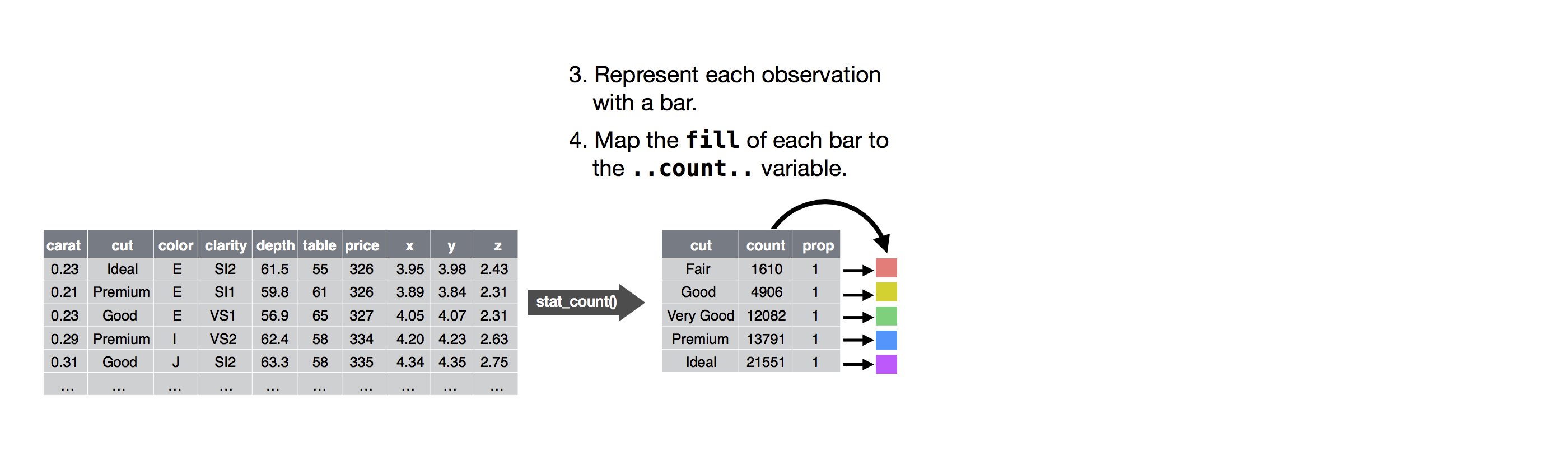
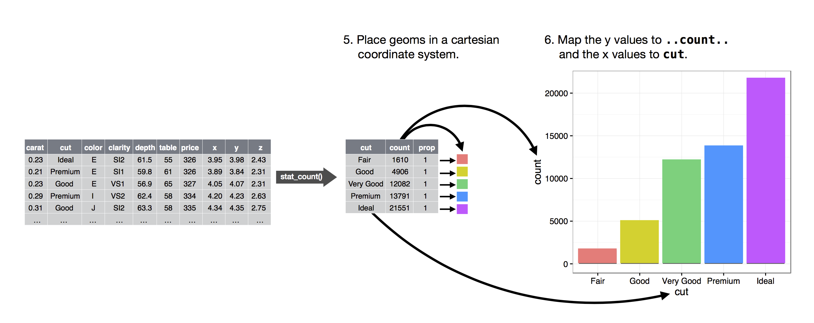
The algorithm used to calculate new values for a graph is chosen a stat, short for statistical transformation. The effigy below describes how this process works with geom_bar().
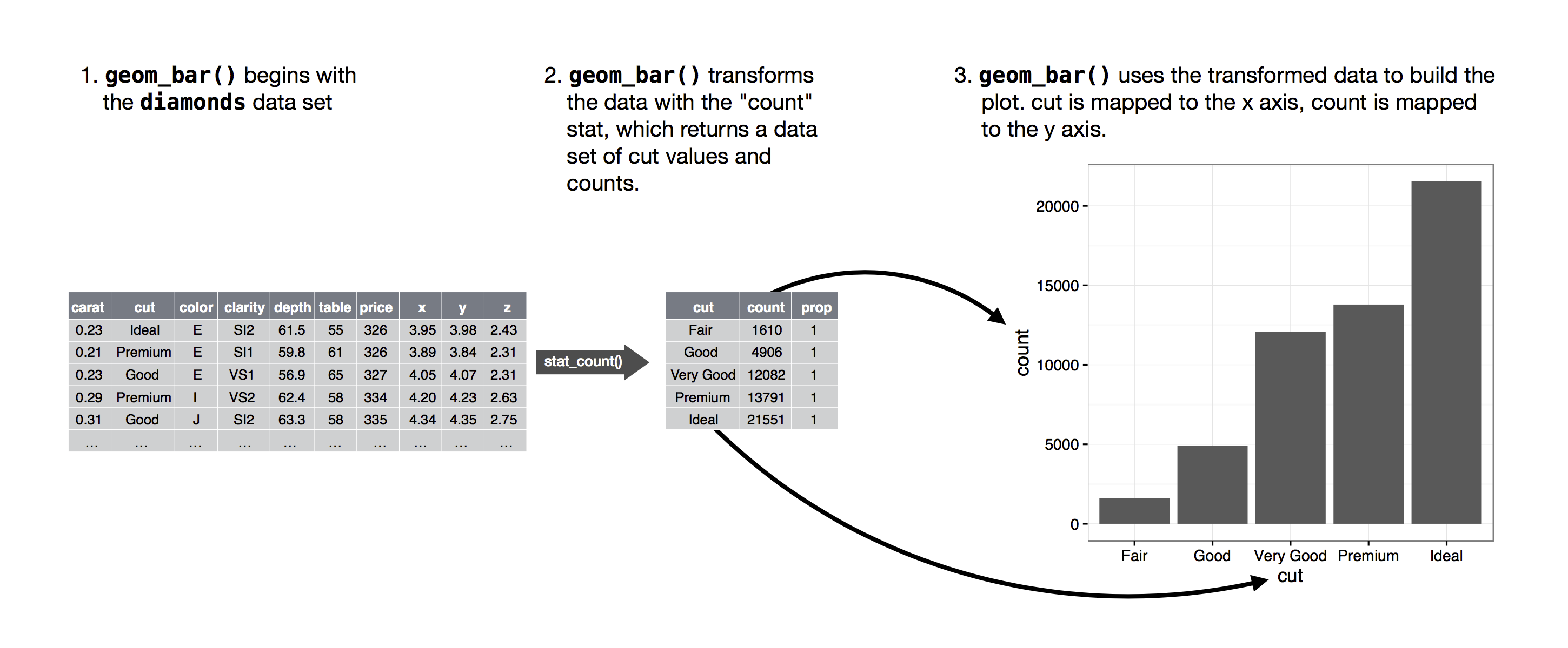
You can larn which stat a geom uses by inspecting the default value for the stat statement. For example, ?geom_bar shows that the default value for stat is "count", which means that geom_bar() uses stat_count(). stat_count() is documented on the same page equally geom_bar(), and if you scroll down you can find a section chosen "Computed variables". That describes how it computes ii new variables: count and prop.
You can more often than not employ geoms and stats interchangeably. For example, you can recreate the previous plot using stat_count() instead of geom_bar():
ggplot (information = diamonds ) + stat_count (mapping = aes (x = cut ) ) 
This works because every geom has a default stat; and every stat has a default geom. This means that you lot can typically use geoms without worrying well-nigh the underlying statistical transformation. There are three reasons you might need to use a stat explicitly:
-
Y'all might want to override the default stat. In the code beneath, I change the stat of
geom_bar()from count (the default) to identity. This lets me map the pinnacle of the bars to the raw values of a \(y\) variable. Unfortunately when people talk nearly bar charts casually, they might be referring to this type of bar chart, where the elevation of the bar is already present in the data, or the previous bar chart where the elevation of the bar is generated by counting rows.demo <- tribble ( ~ cut, ~ freq, "Fair", 1610, "Proficient", 4906, "Very Practiced", 12082, "Premium", 13791, "Platonic", 21551 ) ggplot (data = demo ) + geom_bar (mapping = aes (10 = cutting, y = freq ), stat = "identity" )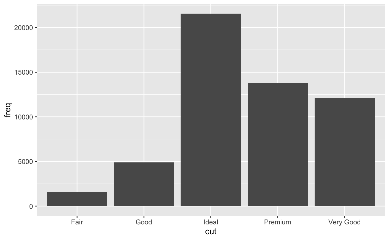
(Don't worry that you haven't seen
<-ortribble()earlier. Yous might be able to estimate at their pregnant from the context, and you'll learn exactly what they exercise shortly!) -
You might want to override the default mapping from transformed variables to aesthetics. For example, you might desire to display a bar chart of proportion, rather than count:
ggplot (data = diamonds ) + geom_bar (mapping = aes (x = cut, y = stat ( prop ), group = 1 ) )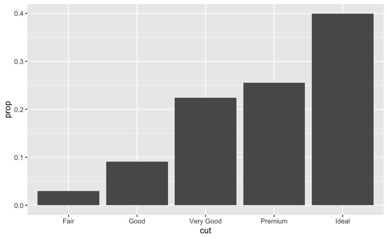
To find the variables computed by the stat, look for the help section titled "computed variables".
-
You lot might want to draw greater attending to the statistical transformation in your lawmaking. For example, you might use
stat_summary(), which summarises the y values for each unique x value, to describe attention to the summary that you're computing:ggplot (data = diamonds ) + stat_summary ( mapping = aes (10 = cut, y = depth ), fun.min = min, fun.max = max, fun = median )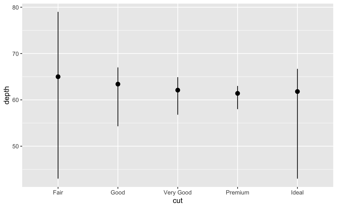
ggplot2 provides over twenty stats for you to utilise. Each stat is a function, so you tin can get help in the usual way, e.grand.?stat_bin. To see a complete listing of stats, attempt the ggplot2 cheatsheet.
Exercises
-
What is the default geom associated with
stat_summary()? How could you rewrite the previous plot to utilize that geom office instead of the stat function? -
What does
geom_col()do? How is information technology different togeom_bar()? -
Almost geoms and stats come in pairs that are near always used in concert. Read through the documentation and make a list of all the pairs. What exercise they take in common?
-
What variables does
stat_smooth()compute? What parameters control its behaviour? -
In our proportion bar chart, we need to set
group = ane. Why? In other words what is the trouble with these ii graphs?ggplot (data = diamonds ) + geom_bar (mapping = aes (x = cutting, y = after_stat ( prop ) ) ) ggplot (data = diamonds ) + geom_bar (mapping = aes (x = cut, fill up = color, y = after_stat ( prop ) ) )
Position adjustments
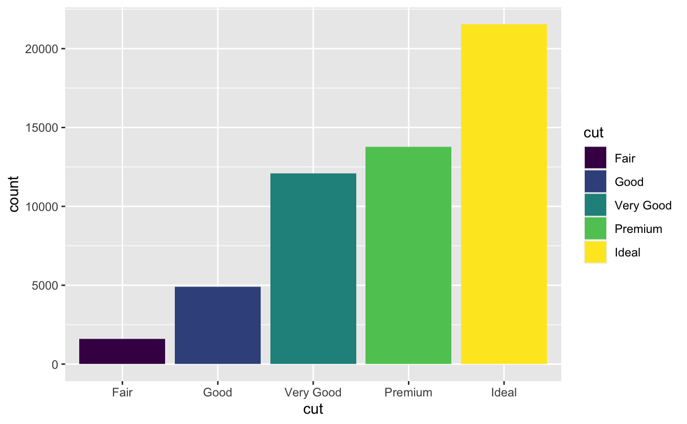
At that place's one more piece of magic associated with bar charts. You can colour a bar chart using either the colour artful, or, more usefully, make full:
ggplot (data = diamonds ) + geom_bar (mapping = aes (x = cut, color = cut ) ) ggplot (data = diamonds ) + geom_bar (mapping = aes (x = cut, make full = cut ) ) 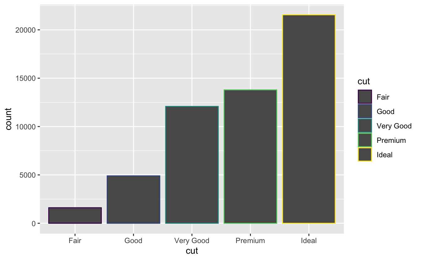
Note what happens if you map the fill aesthetic to another variable, like clarity: the bars are automatically stacked. Each colored rectangle represents a combination of cut and clarity.
ggplot (data = diamonds ) + geom_bar (mapping = aes (x = cut, fill = clarity ) ) 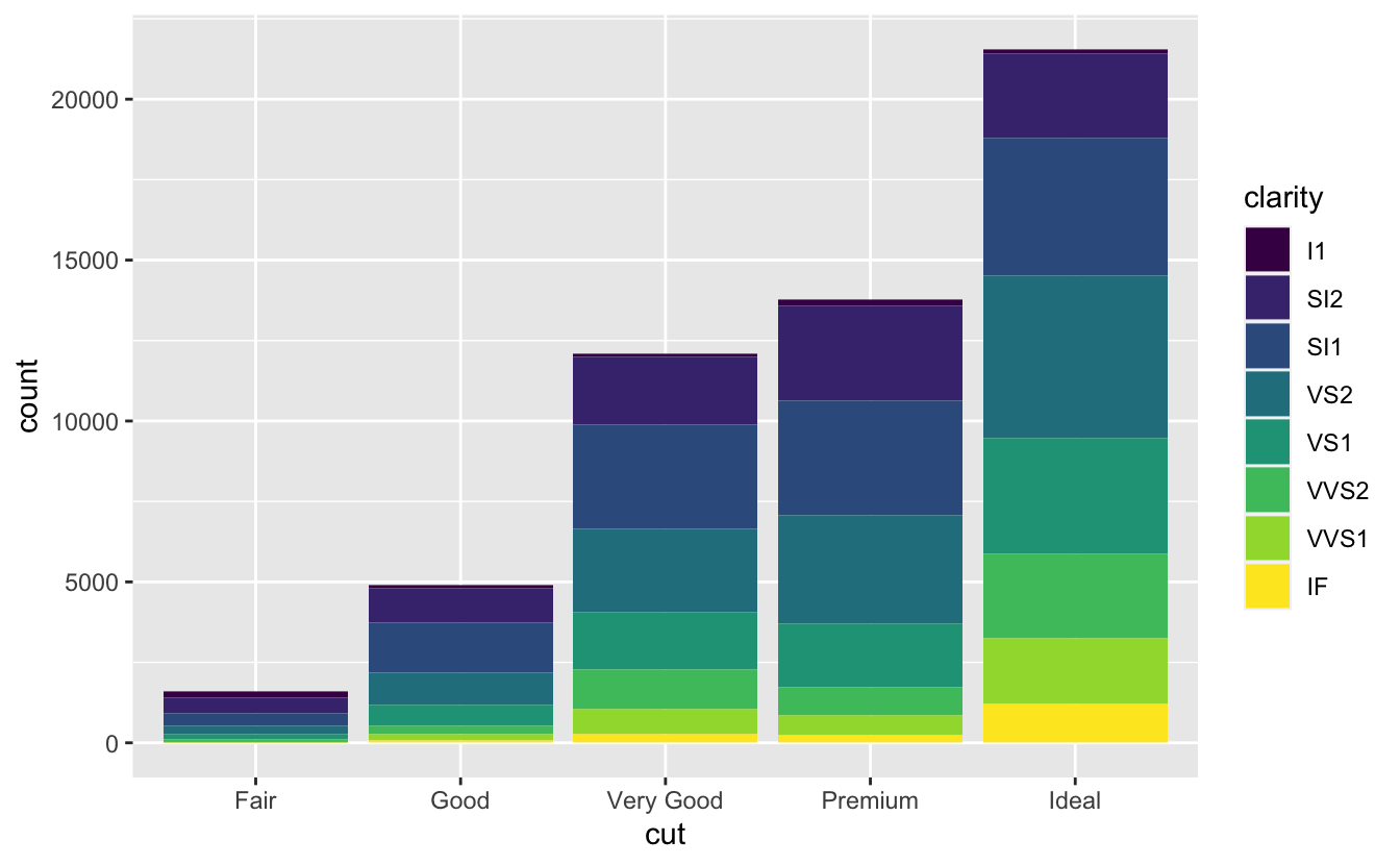
The stacking is performed automatically by the position adjustment specified by the position argument. If you don't want a stacked bar chart, you can apply one of three other options: "identity", "dodge" or "fill up".
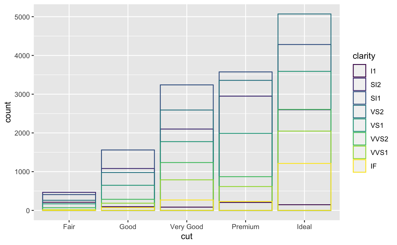
-
position = "identity"will place each object exactly where it falls in the context of the graph. This is not very useful for confined, because it overlaps them. To come across that overlapping we either need to make the bars slightly transparent by settingalphato a small value, or completely transparent by settingfill = NA.ggplot (information = diamonds, mapping = aes (x = cut, fill = clarity ) ) + geom_bar (alpha = 1 / v, position = "identity" ) ggplot (data = diamonds, mapping = aes (ten = cut, colour = clarity ) ) + geom_bar (fill = NA, position = "identity" )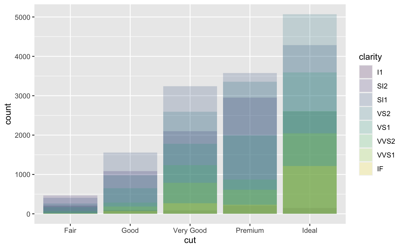
The identity position adjustment is more useful for 2d geoms, like points, where it is the default.
-
position = "fill"works similar stacking, only makes each set of stacked bars the same height. This makes it easier to compare proportions across groups.ggplot (information = diamonds ) + geom_bar (mapping = aes (x = cut, fill = clarity ), position = "make full" )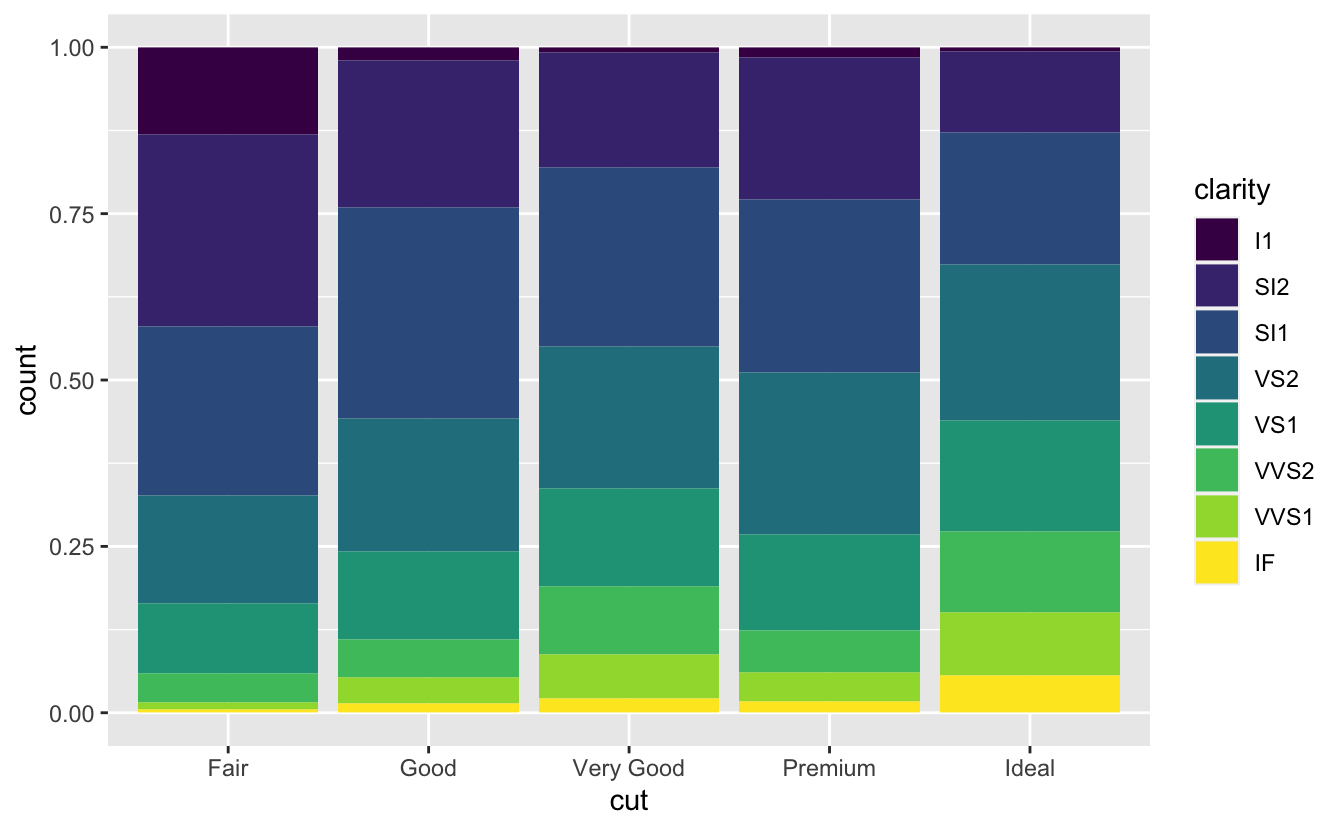
-
position = "dodge"places overlapping objects directly beside one another. This makes it easier to compare private values.ggplot (data = diamonds ) + geom_bar (mapping = aes (x = cut, make full = clarity ), position = "dodge" )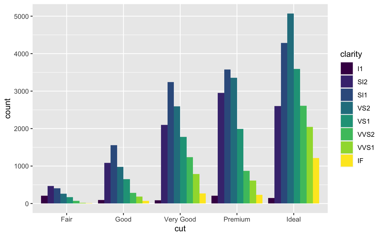
There'south one other type of adjustment that'southward not useful for bar charts, but it can be very useful for scatterplots. Recall our start scatterplot. Did you detect that the plot displays only 126 points, fifty-fifty though at that place are 234 observations in the dataset?

The values of hwy and displ are rounded then the points appear on a filigree and many points overlap each other. This problem is known as overplotting. This organization makes it hard to run into where the mass of the data is. Are the data points spread equally throughout the graph, or is there one special combination of hwy and displ that contains 109 values?
You lot can avoid this gridding by setting the position adjustment to "jitter". position = "jitter" adds a small-scale amount of random noise to each point. This spreads the points out considering no two points are probable to receive the same amount of random noise.
ggplot (information = mpg ) + geom_point (mapping = aes (x = displ, y = hwy ), position = "jitter" ) 
Calculation randomness seems similar a strange style to improve your plot, just while it makes your graph less accurate at pocket-size scales, it makes your graph more revealing at large scales. Because this is such a useful performance, ggplot2 comes with a shorthand for geom_point(position = "jitter"): geom_jitter().
To learn more nigh a position adjustment, look up the help page associated with each aligning: ?position_dodge, ?position_fill, ?position_identity, ?position_jitter, and ?position_stack.
Exercises
-
What is the trouble with this plot? How could you improve it?
ggplot (information = mpg, mapping = aes (x = cty, y = hwy ) ) + geom_point ( )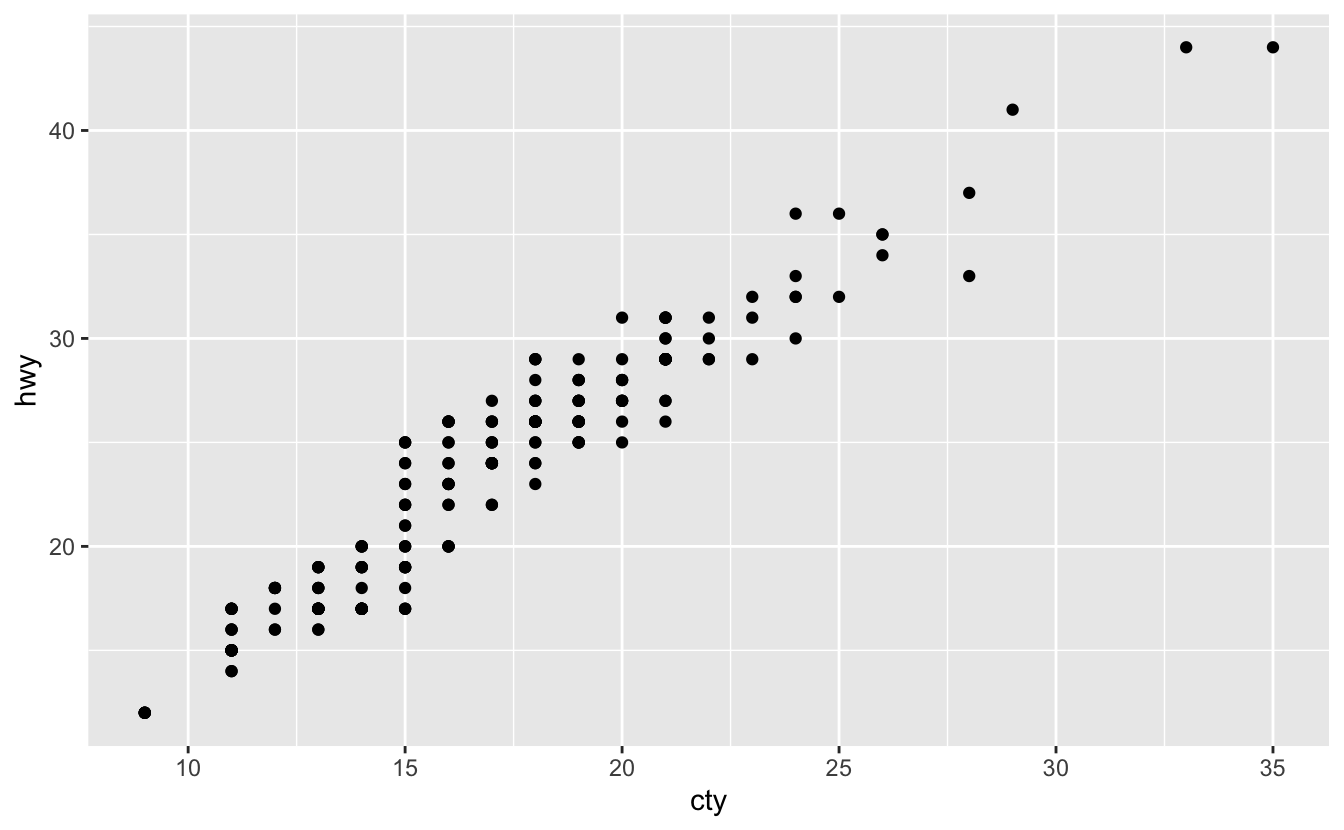
-
What parameters to
geom_jitter()control the corporeality of jittering? -
Compare and contrast
geom_jitter()withgeom_count(). -
What's the default position adjustment for
geom_boxplot()? Create a visualisation of thempgdataset that demonstrates it.
Coordinate systems
Coordinate systems are probably the virtually complicated office of ggplot2. The default coordinate system is the Cartesian coordinate organisation where the 10 and y positions act independently to make up one's mind the location of each point. There are a number of other coordinate systems that are occasionally helpful.
-
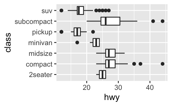
coord_flip()switches the x and y axes. This is useful (for example), if yous want horizontal boxplots. Information technology's also useful for long labels: it'due south difficult to get them to fit without overlapping on the ten-centrality.ggplot (data = mpg, mapping = aes (10 = course, y = hwy ) ) + geom_boxplot ( ) ggplot (data = mpg, mapping = aes (ten = form, y = hwy ) ) + geom_boxplot ( ) + coord_flip ( )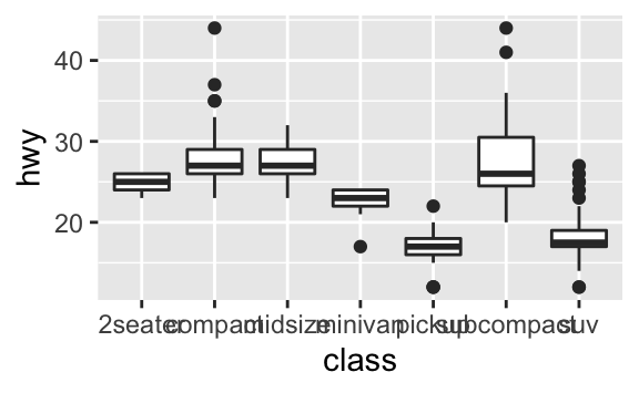
-
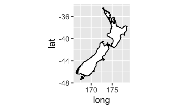
coord_quickmap()sets the aspect ratio correctly for maps. This is very important if you lot're plotting spatial data with ggplot2 (which unfortunately we don't have the space to cover in this book).nz <- map_data ( "nz" ) ggplot ( nz, aes ( long, lat, group = grouping ) ) + geom_polygon (fill = "white", colour = "black" ) ggplot ( nz, aes ( long, lat, group = group ) ) + geom_polygon (fill up = "white", colour = "black" ) + coord_quickmap ( )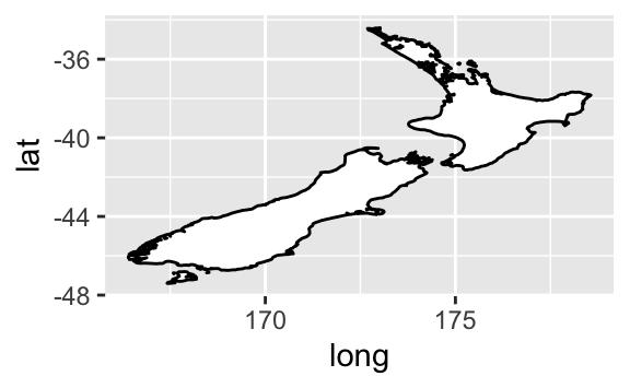
-
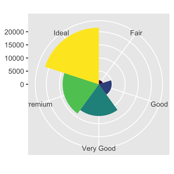
coord_polar()uses polar coordinates. Polar coordinates reveal an interesting connexion betwixt a bar chart and a Coxcomb chart.bar <- ggplot (data = diamonds ) + geom_bar ( mapping = aes (10 = cut, fill = cut ), bear witness.legend = Fake, width = 1 ) + theme (aspect.ratio = 1 ) + labs (ten = Null, y = NULL ) bar + coord_flip ( ) bar + coord_polar ( )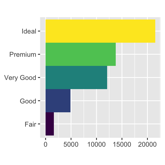
Exercises
-
Turn a stacked bar chart into a pie chart using
coord_polar(). -
What does
labs()practise? Read the documentation. -
What's the deviation betwixt
coord_quickmap()andcoord_map()? -
What does the plot below tell yous almost the relationship between city and highway mpg? Why is
coord_fixed()of import? What doesgeom_abline()do?ggplot (data = mpg, mapping = aes (x = cty, y = hwy ) ) + geom_point ( ) + geom_abline ( ) + coord_fixed ( )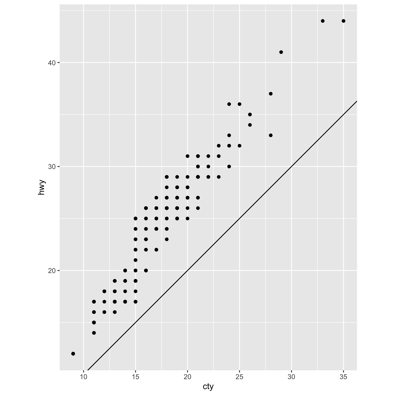
The layered grammer of graphics
In the previous sections, you learned much more how to make scatterplots, bar charts, and boxplots. Yous learned a foundation that y'all can use to brand any type of plot with ggplot2. To see this, let's add position adjustments, stats, coordinate systems, and faceting to our lawmaking template:
ggplot(information = <DATA>) + <GEOM_FUNCTION>( mapping = aes(<MAPPINGS>), stat = <STAT>, position = <POSITION> ) + <COORDINATE_FUNCTION> + <FACET_FUNCTION> Our new template takes seven parameters, the bracketed words that announced in the template. In exercise, you lot rarely need to supply all 7 parameters to brand a graph considering ggplot2 will provide useful defaults for everything except the data, the mappings, and the geom function.
The seven parameters in the template etch the grammar of graphics, a formal organisation for building plots. The grammar of graphics is based on the insight that you can uniquely describe any plot as a combination of a dataset, a geom, a set of mappings, a stat, a position adjustment, a coordinate system, and a faceting scheme.
To come across how this works, consider how you could build a bones plot from scratch: you could start with a dataset and then transform it into the information that you want to display (with a stat).
Next, you could cull a geometric object to represent each observation in the transformed information. You could then use the aesthetic properties of the geoms to correspond variables in the information. You would map the values of each variable to the levels of an artful.
You'd and so select a coordinate system to place the geoms into. You'd use the location of the objects (which is itself an aesthetic property) to display the values of the x and y variables. At that indicate, you lot would accept a consummate graph, simply yous could further adjust the positions of the geoms within the coordinate system (a position adjustment) or dissever the graph into subplots (faceting). You could also extend the plot by adding one or more additional layers, where each additional layer uses a dataset, a geom, a set of mappings, a stat, and a position adjustment.
You lot could utilize this method to build any plot that you imagine. In other words, y'all tin can use the code template that you've learned in this chapter to build hundreds of thousands of unique plots.
Is Guess = Read Default for Geom = Checkpoint
Source: https://r4ds.had.co.nz/data-visualisation.html
0 Response to "Is Guess = Read Default for Geom = Checkpoint"
Post a Comment